You can use this ramp up trick to apply a phasing profile to planned expenditure but I am illustrating it here to model the monthly delivery of planned savings. In the NHS we tend to refer to savings as either QIPP (Quality, Innovation, Productivity and Prevention) or CIP (Cost Improvement Program) depending on whether you have a commissioner or provider focus.
Ideally an organsiation would start planning its efficiency program long before the new year starts and so you might be able to assume that your savings schemes will be fully fledged and able to deliver their full potential from M1 and in that case you wouldn’t need to consider modelling a ramp up. In my experience however, there are normally a set of less well developed QIPP schemes that need a little bedding in to fully develop their savings potential. It is for these schemes that you might like to use Excel to help you model the rate of delivery.
I’ve attached a working spreadsheet example that enables you to play around and experiment with different ramp up profiles. You can also apply seasonality to create a custom ramp up profile and switch between a fixed annual target or not.
Here’s a description of the profiles used in the workbook, which might help you improve your Excel modelling skills.

No ramp-up = delivery at full potential from M1 Linear ramp-up = you build to the full monthly delivery at a constant rate. So by M6 you will delivery 50% of the planned monthly savings and 100% by M12 Slow ramp-up = slow to develop but rate of delivery increases with time Fast ramp-up = as with slow ramp-up but it happens faster
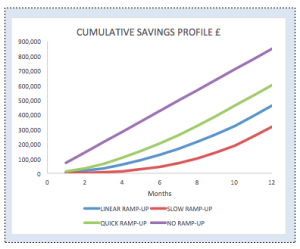
I’ve illustrated this for a QIPP scheme that has the potential to deliver £848,000 worth of savings over the full year. If I don’t fix the outturn you can clearly see that if I show a slow ramp up my savings at year end will be considerably less (£320k) than the full year effect (FYE), in fact that is the case for all profiles other than “No ramp-up”.

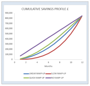
We could alternatively fix the modelling, so that regardless of ramp-up profile, the cumulative saving at year end is fixed, in this case at £848,000. This might not seem terribly realistic, especially when you are comparing profiles but it depends what you are trying to achieve. At the long term planning stage you might say, “we need to achieve £x m efficiency in order to break even”, in that case you could use the fixed outturn position to determine how the monthly challenge increases as we slow down the rate of delivery.

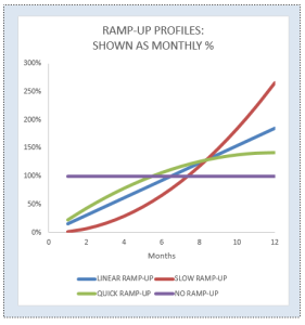
The third chart shows the monthly impact and its clear that for a slow ramp-up you would need to deliver more than 2.5 times the savings at M12 than you would for the No ramp-up scenario.
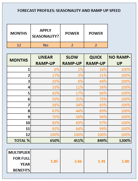
This requires the use of a multiplier to ensure that the cumulative position always comes to 100% of the planned savings.

I would encourage you to download the workbook and play around to see how the modelling works. The orange shaded cells are designed to accept user input so you can dabble with various options.
The power values start at 2, so it is initially modelling quadratic growth but you could switch to cubic and so on.
Here’s the example spreadsheet: Forecast Ramp Up Models
