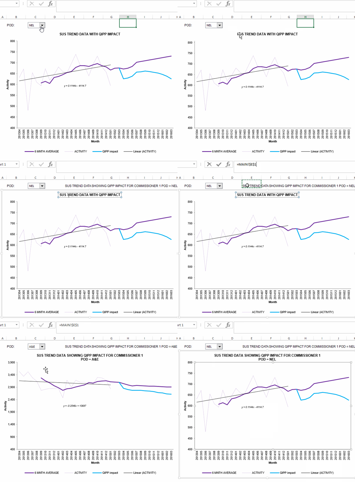
The ability to use formulas in Excel chart titles is very limited and so most people tend to hard code their chart titles. The only formula you can use in the chart title is one that references another cell, for example =$C$1

That does enable you to create a dynamic chart title though - just make sure all the formulaic wizardry occurs in the cell you’ve referenced.

In the animation below I’ve used an example chart from a previous post on linear forecasting. I initially used a static chart title but as my chart was dynamic and linked to a drop down box that enabled me to select different PODs to display, I ideally wanted my chart title to reflect this.

The stages are:

1. Write a formula in a cell that generates the desired chart title
2. You can hide this cell, put it on a different sheet or just turn the font colour to white so that it doesn’t clutter your worksheet
3. Click on the chart title so the box appears
4. Click on the formula bar and type = and then point to the cell with your formula in
5. Hit enter

You should now have a dynamic chart title.