Catchy title I think you’ll agree - GETPIVOTDATA click bait if ever I saw it…

I was preparing a pivot table tutorial for my team at work and during my research I discovered a new tip that filled me with total joy!

I was drawing together my notes on the GETPIVOTDATA function (my all time excel favourite) and I was struggling to explain why you can use a cell address to reference a pivot table item but it goes awry when you use the same method to reference a data field.

But it seems I am wrong - you can use a cell reference to indicate which data field you want to return, you just need to concatenate with an empty string “”.

How the GETPIVOTDATA function works

The syntax for the GETPIVOTDATA function is as follows:

GETPIVOTDATA(data\_field, pivot\_table, \[field1, item1, field2, item2\], ...)

It may look complicated but you never have to write it from scratch.

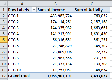
I start by typing = into the cell where I want to retun the value and then click anywhere in my pivot table. This returns the basic but hard-coded formula that I am after.

=GETPIVOTDATA("Sum of Income",$a$1,"CCG Code","CCG 1")

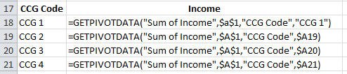
If I drag that formula down it will always return the same value, ie. the sum of Income for CCG 1. However if I change “CCG 1” and reference the cell with the CCG Code in it I can drag down to return the value of interest.

=GETPIVOTDATA("Sum of Income",$a$1,"CCG Code",$A19)

Now if I want to drag the formula right and hope for it to return the activity value rather than the Income value I would need to be able to link the data_field element of my formula to the headers in cell B17 and C17.

If I do that I get an error:

How to Use Cell References for Data Fields with the GETPIVOTDATA function

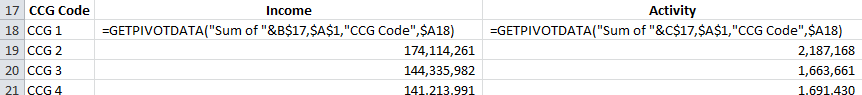
The trick to using a cell reference with Data Fields is to concatenate with an empty string. So in the example above

=GETPIVOTDATA(B$17&"",$a$1,"CCG Code",$A18)

This can then be dragged across and down to give the Income and Activity totals for the relevant pivot items (in this case CCGs).

You may have noticed that this formula now references “Income” without the “Sum of “ prefix that we worked with originally. This works fine until you have multiple aggregate forms of this field in your pivot table. For example you might want to see both the sum and the count of a particular field. If you just reference the field eg “Income” it will only return the Sum of Income.

Therefore, instead of using the empty string I concatenate with the specific aggregation I am after. For example, I will use “Sum of “ or “Count of “ and concatenate with the table header.