I’ve just spent 2 hours with our DBA trying to force SQL to apply the 80/20 rule to a massive data source. I’m so pleased with the result that I have to write it up as a tutorial even though it is not technically an excel solution. In my defence, I will use the output in excel and the SQL trick will enable me to play with manageable volumes rather than gazillions of records. Besides, it is a totally exciting solution and I can’t resist sharing.
The 80/20 Rule or Pareto Principle
The 80/20 rule or Pareto principle is sometimes called the law of the vital few. It is terribly useful in business and analysis in general as it enables you to focus your minimal efforts in the area which will make the biggest difference. Using this rule can turn you into a seriously efficient and effective analyst. Without this rule you run the risk of being run ragged analysing trivia.
The basis is that 80% of the results can be explained by 20% of the inputs, so for example, 20% of company’s customers generate 80% of the revenue. Quite often the ratios can be more skewed e.g. 99% of all complaints generated by only 1% of customers but the principle is the same.
With the two examples above, the run-ragged approach would see you spending a lot of your time responding to and worrying about all your complaints while at the same time attempting to attract your entire customer base to return for a re-order with use of an unfocussed marketing campaign. Alternatively, you could determine whether your 1% of complainants also fell into the 20% of customers who generated 80% of your income. Let’s assume for arguments sake that they didn’t, you could then reprioritise your efforts away from the noise and now focus on the 20% of customers that keep you afloat.
If we are looking for NHS examples:
- The bulk of a hospitals expenditure (80%) is related to a relatively small proportion of patients (20%).
- Most GP appointments are consumed by a small proportion of patients – the chronically sick.
Using the 80/20 Rule to focus Analytical Efforts
My analytical challenge is to amend the monthly income estimate based on some last minute trend data that I have access to.
The reporting estimate has shed loads of data, with each row comprised of hospital site code, specialty code, POD, HRG and commissioner code. The data is a profiled estimate based on the actual activity achieved over the previous months. It includes piffling volume records where perhaps a single activity record in the past 6 months is split into a possible 0.166666 activities estimated for M7.
I need to increase or decrease this estimate based on a trend I can see from another more recent activity source.
Given that I need to take this estimate, then apply a scaling with the output on an excel file (this is how our adjustment process works), I really don’t want to be messing around with many thousands of records, changing an activity estimate of 0.166666 to a far more accurate but equally inconsequential 0.183333
That’s where the 80/20 rule comes into its own. I reckon that I can trim down the volume of data in the estimate file to about 20% of its full size and still have records that contribute in the region of 80% of the value. If I focus my efforts here I can save a lot of time and potential for error that arises when you deal with excessive volumes.
How would I do this in Excel?
This illustration shows an extract of data from my original estimates table (on the left), I’ve coloured it to represent the 4 different partitions I’m interested in, for each unique Site/POD/Spec that exists.
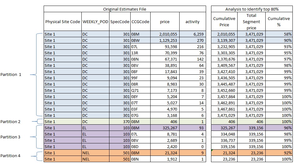
There are 21 rows in the original data with a total value of £3.8m.
On the right I have done a bit of analysis to show the cumulative total by partition and then the Cumulative % by Partition. In order to do this I have had to sort the data in descending order of price by partition and then work out the running total for each.
I’ve dragged the colouring across to show the rows that I want to retain on the basis that they contribute to at least 80% of the total value of each partition.
This second set of data has only 5 rows but still contributes to £3.5m
In 80/20 speak, 23% of the data contribute to 90% of the value. That’s pretty good!
How to use the 80/20 rule in SQL Server
My SQL skills are fairly rudimentary so I’m going to explain the process step by step so I have a chance of remembering what and why we did what we did. There may be better ways to do this, if so shout up in the comments section – I like to learn.
First of all, my script is riddled with cte scripts. That stands for common table expression and basically allows you to create a temporary table, on the fly, that you can reference within your query. A cte isn’t stored and lives only as long as the query.
Step 1 – Summarise the Original Estimate Data
I only want selected PODs and specialties in my extract and I want to group my detail PODs to a higher level grouping eg. OPFAMPCL and OPFASPCL to Outpatients.
The estimates table holds all the historic estimates as well so the first cte, called cte_max_month, returns the maximum and therefore latest month’s estimate. I use this in the second cte called cte_POD.
The 3rd CTE called cte_All just aggregates at my new higher level WEEKLY_POD to ensure I have only one record returned for each unique level of detail.
with

cte\_max\_month as (

select max(month) maxm
from
\[BH\_SLAM\_STAGE\].\[dbo\].\[QVD\_Income\_Estimate\_1718\]
),

cte\_POD as (

SELECT
\[Physical Site Code\]
,Case
when \[POD\] in ('NAFF','OPFAMPCL','OPFASPCL','OPFUPMPCL','OPFUPSPCL','OPPROC') then 'Outpatients'
else \[POD\]
end as WEEKLY\_POD
,\[SpecCode\]
,\[CCGCode\]
,sum(\[priceactual\]) price
,sum(\[activityactual\]) activity

FROM \[BH\_SLAM\_STAGE\].\[dbo\].\[QVD\_Income\_Estimate\_1718\] est

left join cte\_max\_month on est.month = cte\_max\_month.maxm

where POD in ('DC','EL','NAFF','OPFAMPCL','OPFASPCL','OPFUPMPCL','OPFUPSPCL','OPPROC','NEL')
and \[SpecCode\] not in ('650','812')
and month = maxm

group by
\[Physical Site Code\]
,\[POD\]
,\[SpecCode\]
,\[CCGCode\]
),

cte\_All as (
SELECT
\[Physical Site Code\]
,WEEKLY\_POD
,\[SpecCode\]
,\[CCGCode\]
,sum(\[price\]) price
,sum(\[activity\]) activity

FROM cte\_POD

group by
\[Physical Site Code\]
,\[WEEKLY\_POD\]
,\[SpecCode\]
,\[CCGCode\]
)
If I were to return the output of cte_All it would look something like the left hand section of the partition illustration shown above.
Step 2 – Use over(Partition by) to insert a Running Total and a Partition Total
At this stage we begin to build on the summary table cte_All and add a series of columns that will help identify the top 80%.
It utilises OVER(Partition by).
OVER allows you to aggregate data and apply detail alongside it
So
Select
sum(price) over() as value
,\[Physical Site Code\]
,WEEKLY\_POD
,\[SpecCode\]
,\[CCGCode\]

from cte\_All
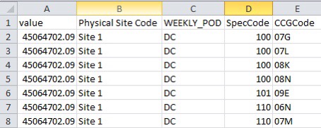
Returns all the detail from cte_ALL but the first column holds the total estimate value for the entire file.
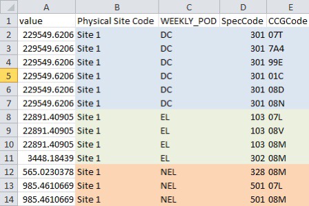
If we then use OVER(PARTITION BY) we can add similar aggregate data to subsets of the detail.
In this case I want to split my data into partitions that correspond to unique combinations of SITE/POD/Spec
Select
sum(price) over (partition by \[Physical Site Code\], WEEKLY\_POD, \[SpecCode\]) as value
,\[Physical Site Code\]
,WEEKLY\_POD
,\[SpecCode\]
,\[CCGCode\]

from cte\_All
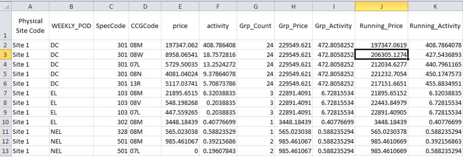
If you also add ORDER BY in the syntax you can use it to return a running total.
So while this script returns the total value for each partition:
sum(price) over(partition by \[Physical Site Code\], WEEKLY\_POD, \[SpecCode\]) as Grp\_Price
This script returns the running total for each partition:
sum(price) over(partition by \[Physical Site Code\], WEEKLY\_POD, \[SpecCode\] order by price desc) as Running\_Price
Here’s the next stage of my script:
cte\_Groups as (
select
\[Physical Site Code\]
,WEEKLY\_POD
,\[SpecCode\]
,\[CCGCode\]
,price
,activity
,count(\*) over(partition by \[Physical Site Code\], WEEKLY\_POD, \[SpecCode\]) as Grp\_Count
,sum(price) over(partition by \[Physical Site Code\], WEEKLY\_POD, \[SpecCode\]) as Grp\_Price
,sum(activity) over(partition by \[Physical Site Code\], WEEKLY\_POD, \[SpecCode\]) as Grp\_Activity
,sum(price) over(partition by \[Physical Site Code\], WEEKLY\_POD, \[SpecCode\] order by price desc) as Running\_Price
,sum(activity) over(partition by \[Physical Site Code\], WEEKLY\_POD, \[SpecCode\] order by activity desc) as Running\_Activity
from cte\_All
)
At this point I am starting to get data that looks useful to me. If this was in excel I would very easily be able to calculate the cumulative percentages and work out a way to filter out the ones I considered significant.
Step 3 – Tidy up the table to remove future Divide by Zero errors
I freely admit to not understanding this stage very well. In step 4 we were getting some divide by zero errors and this step just forces the group totals to have a value.
I’m sure this could be refined. In some way.
cte\_cte\_Filter as (

select
\[Physical Site Code\]
,WEEKLY\_POD
,\[SpecCode\]
,\[CCGCode\]
,price
,activity
,Grp\_Count
,iif(Grp\_Price = 0, 1, Grp\_Price) as Grp\_Price
,iif(Grp\_Activity = 0, 1, Grp\_Activity) as Grp\_Activity
,Running\_Price
,Running\_Activity
from cte\_Groups
)
Step 4 – Add Cumulative Proportion Columns
cte\_Portions as (

select
\[Physical Site Code\]
,WEEKLY\_POD
,\[SpecCode\]
,\[CCGCode\]
,price
,activity
,Grp\_Count
,Running\_Price
,Grp\_Price
,1.0 \* Running\_Price / Grp\_Price as Portion\_Pct\_Price
,1.0 \* isnull(Running\_Activity, 0) / Grp\_Activity as Portion\_pct\_Activity

from cte\_cte\_Filter
)
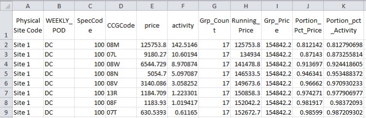
In this extract we can see that the very first record contributes to more than 80% of the value of DC for Spec Code 100
Step 5 – Using SQL Lead and Lag functions to Identify at least 80% of data by Value
In the table above, we could return the correct subset by using where Portion_Pct_Price <= 0.8
However, there are many cases where two or more CCG’s have a significant contribution eg:
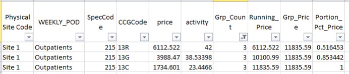 In this example 13R contributes to 51.6% and so would be captured by the Portion_Pct_Price <= 0.8 filter.
The next CCG 13G now brings the cumulative Portion_Pct_Price to 85.3% and so would not meet the <0.8 filter.
In order to ensure that at least 80% is captured we use the LEAD function to reveal information about the next record in the dataset and the LAG function that reveals the detail of the previous dataset. In this case I want to return values where the cumulative % is less than 80% and where the cumulative % is greater than 80% but the previous value was less than 80%.
Here’s the script that does that along with the final output query:
cte\_Lead as (
--this query determines the cumulative portion % for the next (lead) and the previous (lag) record by partition
select
\[Physical Site Code\]
,WEEKLY\_POD
,\[SpecCode\]
,\[CCGCode\]
,price
,activity
,Grp\_Count
,Running\_Price
,Grp\_Price
,Portion\_Pct\_Price
,Portion\_pct\_Activity
,lead(Portion\_Pct\_Price, 1) over(partition by \[Physical Site Code\], WEEKLY\_POD, \[SpecCode\] order by price desc) as Nxt\_Portion\_Pct\_Price
,lead(Portion\_pct\_Activity, 1) over(partition by \[Physical Site Code\], WEEKLY\_POD, \[SpecCode\] order by price desc) as Nxt\_Portion\_pct\_Activity
,lag(Portion\_Pct\_Price, 1) over(partition by \[Physical Site Code\], WEEKLY\_POD, \[SpecCode\] order by price desc) as Pre\_Portion\_Pct\_Price
,lag(Portion\_pct\_Activity, 1) over(partition by \[Physical Site Code\], WEEKLY\_POD, \[SpecCode\] order by price desc) as Pre\_Portion\_pct\_Activity

from cte\_Portions
)

--output
select \*
from cte\_Lead
where Portion\_Pct\_Price <= 0.8

union all

select \*
from cte\_Lead
where (Portion\_Pct\_Price > 0.8 and Pre\_Portion\_Pct\_Price < 0.8)
or (Portion\_Pct\_Price > 0.8 and (Pre\_Portion\_Pct\_Price) is null)
Outstanding Issues to Consider
At the moment my process assumes all my financial values are positive. If I had significant credits in my dataset I would be ignoring them. That might not be appropriate for your application so think carefully about it – perhaps you could let me know how you solved it.