The sumproduct function is one of the most useful and powerful features of excel but the online help available from microsoft is unfortunately pretty poor.
It works as an advanced form of the SUMIF formula where you can sum a range of values based on a number of different criteria.
Here is the simple formula layout or syntax:
=SUMPRODUCT((Condition 1)\*(The range to sum))
or slightly more complex:
=SUMPRODUCT((Condition 1)\*(Condition 2)\*(The range to sum)
the “*” symbol between conditions represents an AND a “+” symbol would represent an OR.
Here is a simple example, of a schools course grades displayed in the following spreadsheet table
You will probably want to summarise this to show the total number of students passing the course in each grade.
This makes use of the simple SUMPRODUCT formula in cell F2:
=SUMPRODUCT(($B$2:$B$15=E2)\*($C$2:$C$15))
the use of absolute referencing here enables the formula to be copied all the way down the table.
In English the spreadsheet formula reads:
Sum the results in column C where the values in column B = “A”
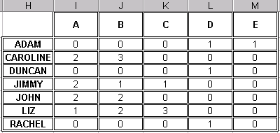
Moving on to a slightly more complex example, we could increase the summary table to show each students performance across the different grades.
This requires the addition of another condition – namely STUDENT equals.
The spreadsheet formula in cell I2, which can again be copied across is:
=SUMPRODUCT(($B$2:$B$15=I$1)\*($A$2:$A$15=$H2)\*($C$2:$C$15))
In English the spreadsheet formula reads:
Sum the results in column C where the grades = “A” and where the student = “Adam”
To see these powerful excel functions in action and utilising the Condition 1 OR condition 2 terminology, download my example sumproduct.xls.


