Excel offers a number of conditional IF functions such as COUNTIF and SUMIF which allow you to count or sum a range based on the values in another column. If you have Excel 2007 or later you’ll have the really useful COUNTIFS and SUMIFS functions which allow you to perform multi-condition actions based on the values in multiple columns. If you are looking around for a RANKIF function you are going to be disappointed - Microsoft appear to have missed a trick.
I wanted a RANKIF function the other day when I was reviewing the latest Reference Cost release to enable me to rank all the available hospitals according to their cost (reference cost) for a specific HRG.
If you are using a version of Excel prior to 2007 you will need to use the SUMPRODUCT function to achieve the ranking but if you are using a later version of Excel you have the additional option of using the COUNTIFS function to assist. They both do the same job, but COUNTIFS is slightly easier to understand.
Performing a RANKIF using the SUMPRODUCT function
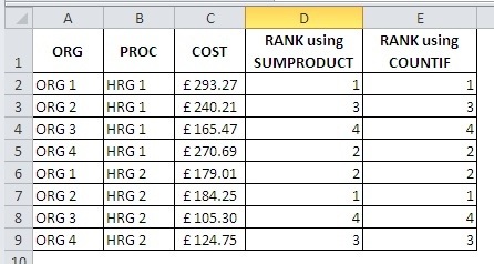
The formula I used to achieve the above ranking was:
=1+SUMPRODUCT(($B$2:$B$12=B2)\*($C$2:$C$12>C2))
Copied down the column it will return the number of organisations for a given HRG which have costs higher than the selected row. Adding 1 to the result just ensures that the highest cost organisation starts with a rank of 1 rather than 0.
With SUMPRODUCT the “*” symbol between conditions represents an AND a “+” symbol would represent an OR.
It’s a little difficult to explain this formula in real terms but the bracketed areas are returning true or false (1 or 0) and the sumproduct multiplies the two arrays together and then adds the results. So in our example of 8 rows, the calculation in cell D2 would be:

And just to reiterate the process, the calculation D3 would be like this:

Performing a RANKIF using the COUNTIFS function
The formula I used to achieve the above ranking was:
= 1+COUNTIFS($B$2:$B$9,B2,$C$2:$C$9,“>”&C2)
This outputs exactly the same result but it is much easier to understand what the formula is doing:
Count the number of entries in column C where the HRG is the same and where the cost is higher than in the current row. Add 1 just to ensure that the highest cost returns 1 rather than 0.
Link to excel 2007 and 97–2003 versions of the RANKIF workbooks (note that the earlier version does not support COUNTIFS).